Rotatory Position Embedding (RoPE)

Introduction

Positional embedding is a crucial part of transformer models such as BERT and GPT. Unlike traditional models such as RNNs or LSTMs that understand the order of input sequences through sequential processing, transformers consider input sequences as unordered sets. This approach improves computational efficiency and overall performance, but it doesn’t account for the natural order of tokens, which is essential for understanding text. This limitation exists because the transformer architecture relies on self-attention mechanisms, which are permutation-invariant. This means they treat all positions equally, regardless of the element arrangement in the sequence. Positional embeddings address this shortcoming by integrating the sequence’s order into the model’s inputs, enabling the model to maintain awareness of token positions. This understanding is essential for language tasks such as translation, generation, and comprehension, where changing the word sequence can drastically change sentence meaning. For example, “The cat sat on the mat” and “The mat sat on the cat” have the exact words but different meanings due to word order.

Transformer models use two primary types of positional embeddings: Absolute and Relative. Absolute positional embeddings assign a unique identifier to each position in a sequence, enabling the model to learn and utilize the absolute position of tokens. On the other hand, relative positional embeddings focus on the distances between pairs of tokens, thereby allowing the model to understand and leverage the relative positioning of tokens within a sequence.

Sinusoidal Positional Encoding

The original transformer model, which was introduced in the paper “Attention is All You Need”, uses sine and cosine functions to create positional embeddings. These embeddings are absolute, which means that each position in the sequence is assigned a unique sinusoidal pattern. This helps the model to effectively differentiate between the tokens and utilize their order.

Sine and cosine positional embeddings are calculated as follows for each position \(pos\) and each dimension \(i\) of the \(d_{model}\)-dimensional token embedding:

This formulation ensures each position \(pos\) in the sequence receives a unique embedding, with the embeddings transitioning smoothly across positions.

Consider a scenario where we have a sequence of words and we wish to encode the position of each word. The model’s dimension \(d_{model}\) is 4 for simplicity.

Step-by-Step Calculation for a Single Position

• Position 1, Dimension 0 and 1: For the first position (\(pos = 0\)) and the first dimension (\(i = 0\)): \(PE_{(0, 0)} = \sin\left(\frac{0}{10000^{0}}\right) = \sin(0) = 0\) \(PE_{(0, 1)} = \cos\left(\frac{0}{10000^{0}}\right) = \cos(0) = 1\)

This process is repeated for each dimension of the embedding, creating a unique blend of sine and cosine values that vary smoothly and predictably across positions.

Code Implementation of Sinusoidal Positional Encoding

import numpy as np

def sinusoidal_positional_encoding(pos, d_model):
    position = np.arange(pos)[:, np.newaxis]
    div_term = np.exp(np.arange(0, d_model, 2) * -(np.log(10000.0) / d_model))
    pe = np.zeros((pos, d_model))
    pe[:, 0::2] = np.sin(position * div_term)
    pe[:, 1::2] = np.cos(position * div_term)
    return pe

• np.arange(pos)[:, np.newaxis]: Creates a column vector with positions from 0 to pos-1.
• div_term: Calculates the denominator for the exponent, scaling down the rate of change for higher dimensions.
• pe[:, 0::2] = np.sin(position * div_term): Assigns the sine values to even indices of the embedding.
• pe[:, 1::2] = np.cos(position * div_term): Assigns the cosine values to odd indices.

This implementation efficiently encodes positional information into a matrix, which can be added to the token embeddings, enriching them with positional context.

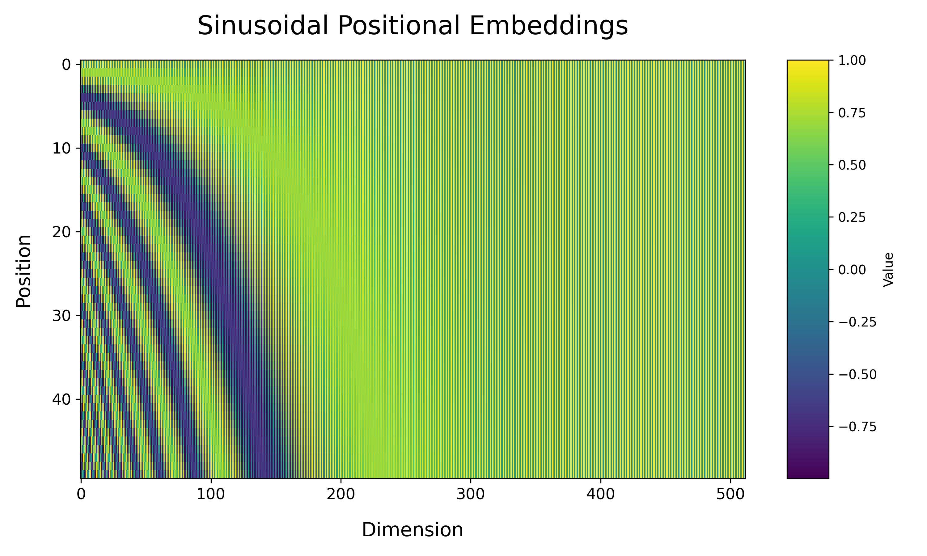
Below visualization show a smooth, wave-like pattern, demonstrating how each position is uniquely encoded yet transitions smoothly to the next.

Despite its effectiveness, sinusoidal positional embeddings have limitations, particularly with longer sequences than those seen during training.

Rotary Positional Embedding (RoPE)

Jianlin Su et al. introduced Rotary Positional Embedding (RoPE) to solve a above problem. RoPE uses a unique method to encode positions by rotating the embedding vectors in a multidimensional space. This is different from sinusoidal embeddings which add fixed wave patterns to the embeddings based on their positions. RoPE uses a rotation matrix to alter the representation of each token in a geometric way, similar to how relationships in physical spaces can be understood through angles and distances. This provides a more natural way to represent sequential information. Sinusoidal embeddings may not be effective over long distances or in complex sequences where the positional relationship is key to interpretation. RoPE’s rotation-based method maintains the relative positional information, making it particularly adept at handling such challenges.

For a given token at position \(pos\), with its embedding vector \(x_{pos}\), RoPE defines a rotation matrix based on the token’s position that encodes the positional information:

Here, \(x_{pos}\) is the original embedding vector, and \(\hat{x}_{pos}\) is a version of \(x_{pos}\) that has been rotated by the angle \(\theta_{pos}\) in the embedding space. This angle is a predetermined function of the position, ensuring a unique rotation for each token.

To illustrate the process more concretely, let’s walk through how RoPE would encode a two-token sequence in a model where embeddings are two-dimensional:

1. Initial Embeddings: Start with the initial embeddings for tokens A and B, \(\vec{x}_A\) and \(\vec{x}_B\), in a 2D space.

2. Positional Rotation: For each token, calculate a rotation angle \(\theta_A\) and \(\theta_B\) based on their respective positions in the sequence.

3. Apply Rotation: Rotate each token’s embedding vector by its corresponding angle. This is done through element-wise multiplication by cosine and sine of the angles.

4. Rotated Embeddings: The new positions \(\vec{x}'_A\) and \(\vec{x}'_B\) now contain both original and relative positional information, enabling the model to understand the sequence order.

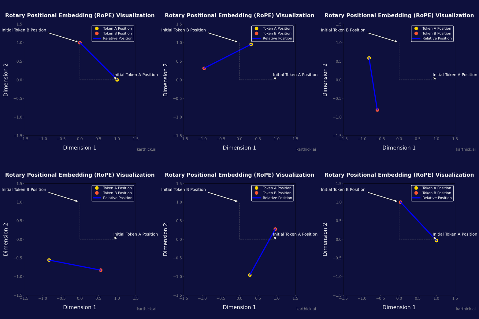
Visualizing RoPE

• Initial Token Positions: The starting points for Token A and Token B.
• Token Rotations: Reflecting the positional encoding process.
• Relative Positioning: The relative distance between Token A and B is preserved post-rotation, signifying the model’s understanding of their order and spacing.

Advantages of RoPE

• Long-Range Context: RoPE adeptly captures relationships between tokens across lengthy sequences, a challenge for conventional positional embeddings.
• Rotation Invariance: By design, RoPE maintains effectiveness irrespective of sequence length, addressing a limitation of sine-cosine embeddings.
• Interpretability: The rotational approach offers an intuitive geometric interpretation of how positional information influences the attention mechanism.

Code Implementation

import torch

def rotary_position_embedding(max_seq_len, dim):
    # Calculate the angle rates based on dimension indices.
    angle_rates = 1 / torch.pow(10000, torch.arange(0, dim, 2).float() / dim)
    # Calculate the angles for each position for half of the dimensions (sine and cosine)
    angles = (torch.arange(max_seq_len).unsqueeze(1) * angle_rates.unsqueeze(0))
    # Cosines and sines of the angles to get the RoPE for each position
    position_encodings = torch.stack((angles.cos(), angles.sin()), dim=2).flatten(1)
    return position_encodings

def apply_rope_embeddings(embeddings, position_encodings):
    # Split the position encodings into cosines and sines
    cos_enc, sin_enc = position_encodings[..., 0::2], position_encodings[..., 1::2]
    # Apply the rotations
    embeddings[..., 0::2] = embeddings[..., 0::2] * cos_enc - embeddings[..., 1::2] * sin_enc
    embeddings[..., 1::2] = embeddings[..., 1::2] * cos_enc + embeddings[..., 0::2] * sin_enc
    return embeddings

batch_size, max_seq_len, dim = 1, 128, 512  # Dimensions for batch size, sequence length, and embedding dimension

# Initialize random embeddings simulating a batch of token embeddings
token_embeddings = torch.randn(batch_size, max_seq_len, dim)

# Generate the position encodings for the sequence
position_encodings = rotary_position_embedding(max_seq_len, dim)

# Apply the RoPE to the token embeddings
rotated_token_embeddings = apply_rope_embeddings(token_embeddings, position_encodings)

The latest LLM models like Mistral and Llama are incorporating RoPE in their architecture. Understanding both the theoretical concepts and practical code implementation will help you to grasp these advanced models. I hope you found this blog informative and enjoyable. If you liked it, follow me on LinkedIn for more posts like this.

Reference

1. Vaswani, Ashish, et al. “Attention Is All You Need.” ArXiv, 2017, /abs/1706.03762. Accessed 5 Apr. 2024.

2. Su, Jianlin, et al. “RoFormer: Enhanced Transformer with Rotary Position Embedding.” ArXiv, 2021, /abs/2104.09864. Accessed 5 Apr. 2024.